| Data Visualization using Matplotlib | 您所在的位置:网站首页 › data visualization programs in python › Data Visualization using Matplotlib |
Data Visualization using Matplotlib
|
Data Visualization is the process of presenting data in the form of graphs or charts. It helps to understand large and complex amounts of data very easily. It allows the decision-makers to make decisions very efficiently and also allows them in identifying new trends and patterns very easily. It is also used in high-level data analysis for Machine Learning and Exploratory Data Analysis (EDA). Data visualization can be done with various tools like Tableau, Power BI, Python. In this article, we will discuss how to visualize data with the help of the Matplotlib library of Python. MatplotlibMatplotlib is a low-level library of Python which is used for data visualization. It is easy to use and emulates MATLAB like graphs and visualization. This library is built on the top of NumPy arrays and consist of several plots like line chart, bar chart, histogram, etc. It provides a lot of flexibility but at the cost of writing more code. InstallationWe will use the pip command to install this module. If you do not have pip installed then refer to the article, Download and install pip Latest Version. To install Matplotlib type the below command in the terminal. pip install matplotlib
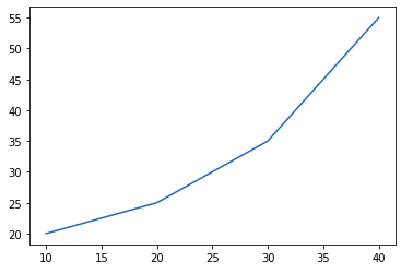
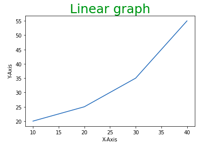
Refer to the below articles to get more information setting up an environment with Matplotlib. Environment Setup for MatplotlibUsing Matplotlib with Jupyter NotebookPyplotPyplot is a Matplotlib module that provides a MATLAB-like interface. Matplotlib is designed to be as usable as MATLAB, with the ability to use Python and the advantage of being free and open-source. Each pyplot function makes some change to a figure: e.g., creates a figure, creates a plotting area in a figure, plots some lines in a plotting area, decorates the plot with labels, etc. The various plots we can utilize using Pyplot are Line Plot, Histogram, Scatter, 3D Plot, Image, Contour, and Polar. After knowing a brief about Matplotlib and pyplot let’s see how to create a simple plot. Example: Python3import matplotlib.pyplot as plt # initializing the datax = [10, 20, 30, 40]y = [20, 25, 35, 55] # plotting the dataplt.plot(x, y) plt.show()Output:
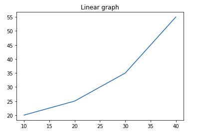
Now let see how to add some basic elements like title, legends, labels to the graph. Note: For more information about Pyplot, refer Pyplot in Matplotlib Adding TitleThe title() method in matplotlib module is used to specify the title of the visualization depicted and displays the title using various attributes. Syntax: matplotlib.pyplot.title(label, fontdict=None, loc=’center’, pad=None, **kwargs) Example: Python3import matplotlib.pyplot as plt # initializing the datax = [10, 20, 30, 40]y = [20, 25, 35, 55] # plotting the dataplt.plot(x, y) # Adding title to the plotplt.title("Linear graph") plt.show()Output:
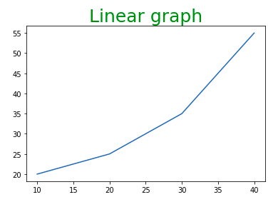
We can also change the appearance of the title by using the parameters of this function. Example: Python3import matplotlib.pyplot as plt # initializing the datax = [10, 20, 30, 40]y = [20, 25, 35, 55] # plotting the dataplt.plot(x, y) # Adding title to the plotplt.title("Linear graph", fontsize=25, color="green") plt.show()Output:
Note: For more information about adding the title and its customization, refer Matplotlib.pyplot.title() in Python Adding X Label and Y LabelIn layman’s terms, the X label and the Y label are the titles given to X-axis and Y-axis respectively. These can be added to the graph by using the xlabel() and ylabel() methods. Syntax: matplotlib.pyplot.xlabel(xlabel, fontdict=None, labelpad=None, **kwargs) matplotlib.pyplot.ylabel(ylabel, fontdict=None, labelpad=None, **kwargs) Example: Python3import matplotlib.pyplot as plt # initializing the datax = [10, 20, 30, 40]y = [20, 25, 35, 55] # plotting the dataplt.plot(x, y) # Adding title to the plotplt.title("Linear graph", fontsize=25, color="green") # Adding label on the y-axisplt.ylabel('Y-Axis') # Adding label on the x-axisplt.xlabel('X-Axis') plt.show()Output:
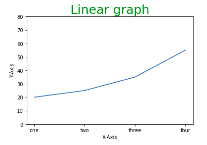
You might have seen that Matplotlib automatically sets the values and the markers(points) of the X and Y axis, however, it is possible to set the limit and markers manually. xlim() and ylim() functions are used to set the limits of the X-axis and Y-axis respectively. Similarly, xticks() and yticks() functions are used to set tick labels. Example: In this example, we will be changing the limit of Y-axis and will be setting the labels for X-axis. Python3import matplotlib.pyplot as plt # initializing the datax = [10, 20, 30, 40]y = [20, 25, 35, 55] # plotting the dataplt.plot(x, y) # Adding title to the plotplt.title("Linear graph", fontsize=25, color="green") # Adding label on the y-axisplt.ylabel('Y-Axis') # Adding label on the x-axisplt.xlabel('X-Axis') # Setting the limit of y-axisplt.ylim(0, 80) # setting the labels of x-axisplt.xticks(x, labels=["one", "two", "three", "four"]) plt.show()Output:
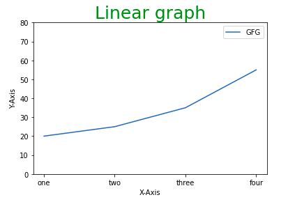
A legend is an area describing the elements of the graph. In simple terms, it reflects the data displayed in the graph’s Y-axis. It generally appears as the box containing a small sample of each color on the graph and a small description of what this data means. The attribute bbox_to_anchor=(x, y) of legend() function is used to specify the coordinates of the legend, and the attribute ncol represents the number of columns that the legend has. Its default value is 1. Syntax: matplotlib.pyplot.legend([“name1”, “name2”], bbox_to_anchor=(x, y), ncol=1) Example: Python3import matplotlib.pyplot as plt # initializing the datax = [10, 20, 30, 40]y = [20, 25, 35, 55] # plotting the dataplt.plot(x, y) # Adding title to the plotplt.title("Linear graph", fontsize=25, color="green") # Adding label on the y-axisplt.ylabel('Y-Axis') # Adding label on the x-axisplt.xlabel('X-Axis') # Setting the limit of y-axisplt.ylim(0, 80) # setting the labels of x-axisplt.xticks(x, labels=["one", "two", "three", "four"]) # Adding legendsplt.legend(["GFG"]) plt.show()Output:
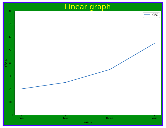
Before moving any further with Matplotlib let’s discuss some important classes that will be used further in the tutorial. These classes are – FigureAxesNote: Matplotlib take care of the creation of inbuilt defaults like Figure and Axes. Figure classConsider the figure class as the overall window or page on which everything is drawn. It is a top-level container that contains one or more axes. A figure can be created using the figure() method. Syntax: class matplotlib.figure.Figure(figsize=None, dpi=None, facecolor=None, edgecolor=None, linewidth=0.0, frameon=None, subplotpars=None, tight_layout=None, constrained_layout=None) Example: Python3# Python program to show pyplot moduleimport matplotlib.pyplot as pltfrom matplotlib.figure import Figure # initializing the datax = [10, 20, 30, 40]y = [20, 25, 35, 55] # Creating a new figure with width = 7 inches# and height = 5 inches with face color as# green, edgecolor as red and the line width# of the edge as 7fig = plt.figure(figsize =(7, 5), facecolor='g', edgecolor='b', linewidth=7) # Creating a new axes for the figureax = fig.add_axes([1, 1, 1, 1]) # Adding the data to be plottedax.plot(x, y) # Adding title to the plotplt.title("Linear graph", fontsize=25, color="yellow") # Adding label on the y-axisplt.ylabel('Y-Axis') # Adding label on the x-axisplt.xlabel('X-Axis') # Setting the limit of y-axisplt.ylim(0, 80) # setting the labels of x-axisplt.xticks(x, labels=["one", "two", "three", "four"]) # Adding legendsplt.legend(["GFG"]) plt.show()Output:
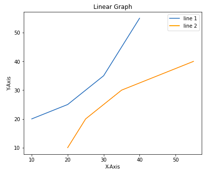
>>> More Functions in Figure Class Axes ClassAxes class is the most basic and flexible unit for creating sub-plots. A given figure may contain many axes, but a given axes can only be present in one figure. The axes() function creates the axes object. Syntax: axes([left, bottom, width, height]) Just like pyplot class, axes class also provides methods for adding titles, legends, limits, labels, etc. Let’s see a few of them – Adding Title – ax.set_title()Adding X Label and Y label – ax.set_xlabel(), ax.set_ylabel()Setting Limits – ax.set_xlim(), ax.set_ylim()Tick labels – ax.set_xticklabels(), ax.set_yticklabels()Adding Legends – ax.legend()Example: Python3# Python program to show pyplot moduleimport matplotlib.pyplot as pltfrom matplotlib.figure import Figure # initializing the datax = [10, 20, 30, 40]y = [20, 25, 35, 55] fig = plt.figure(figsize = (5, 4)) # Adding the axes to the figureax = fig.add_axes([1, 1, 1, 1]) # plotting 1st dataset to the figureax1 = ax.plot(x, y) # plotting 2nd dataset to the figureax2 = ax.plot(y, x) # Setting Titleax.set_title("Linear Graph") # Setting Labelax.set_xlabel("X-Axis")ax.set_ylabel("Y-Axis") # Adding Legendax.legend(labels = ('line 1', 'line 2')) plt.show()Output:
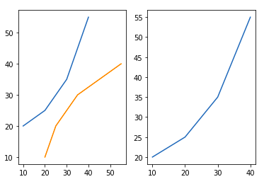
We have learned about the basic components of a graph that can be added so that it can convey more information. One method can be by calling the plot function again and again with a different set of values as shown in the above example. Now let’s see how to plot multiple graphs using some functions and also how to plot subplots. Method 1: Using the add_axes() method The add_axes() method is used to add axes to the figure. This is a method of figure class Syntax: add_axes(self, *args, **kwargs) Example: Python3# Python program to show pyplot moduleimport matplotlib.pyplot as pltfrom matplotlib.figure import Figure # initializing the datax = [10, 20, 30, 40]y = [20, 25, 35, 55] # Creating a new figure with width = 5 inches# and height = 4 inchesfig = plt.figure(figsize =(5, 4)) # Creating first axes for the figureax1 = fig.add_axes([0.1, 0.1, 0.8, 0.8]) # Creating second axes for the figureax2 = fig.add_axes([1, 0.1, 0.8, 0.8]) # Adding the data to be plottedax1.plot(x, y)ax2.plot(y, x) plt.show()Output:
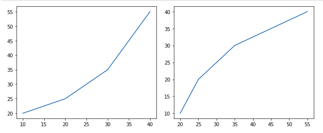
Method 2: Using subplot() method. This method adds another plot at the specified grid position in the current figure. Syntax: subplot(nrows, ncols, index, **kwargs) subplot(pos, **kwargs) subplot(ax) Example: Python3import matplotlib.pyplot as plt # initializing the datax = [10, 20, 30, 40]y = [20, 25, 35, 55] # Creating figure objectplt.figure() # adding first subplotplt.subplot(121)plt.plot(x, y) # adding second subplotplt.subplot(122)plt.plot(y, x)Output:
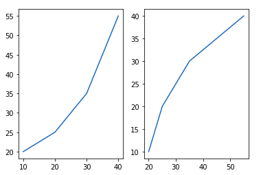
Method 3: Using subplots() method This function is used to create figures and multiple subplots at the same time. Syntax: matplotlib.pyplot.subplots(nrows=1, ncols=1, sharex=False, sharey=False, squeeze=True, subplot_kw=None, gridspec_kw=None, **fig_kw) Example: Python3import matplotlib.pyplot as plt # initializing the datax = [10, 20, 30, 40]y = [20, 25, 35, 55] # Creating the figure and subplots# according the argument passedfig, axes = plt.subplots(1, 2) # plotting the data in the# 1st subplotaxes[0].plot(x, y) # plotting the data in the 1st# subplot onlyaxes[0].plot(y, x) # plotting the data in the 2nd# subplot onlyaxes[1].plot(x, y)Output:
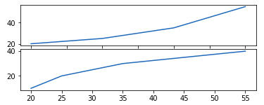
Method 4: Using subplot2grid() method This function creates axes object at a specified location inside a grid and also helps in spanning the axes object across multiple rows or columns. In simpler words, this function is used to create multiple charts within the same figure. Syntax: Plt.subplot2grid(shape, location, rowspan, colspan) Example: Python3import matplotlib.pyplot as plt # initializing the datax = [10, 20, 30, 40]y = [20, 25, 35, 55] # adding the subplotsaxes1 = plt.subplot2grid ((7, 1), (0, 0), rowspan = 2, colspan = 1) axes2 = plt.subplot2grid ((7, 1), (2, 0), rowspan = 2, colspan = 1) # plotting the dataaxes1.plot(x, y)axes2.plot(y, x)Output:
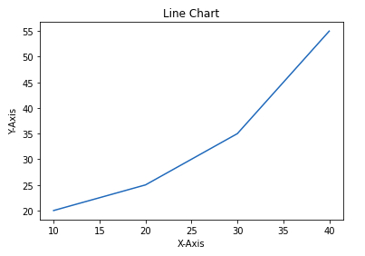
Matplotlib supports a variety of plots including line charts, bar charts, histograms, scatter plots, etc. We will discuss the most commonly used charts in this article with the help of some good examples and will also see how to customize each plot. Note: Some elements like axis, color are common to each plot whereas some elements are pot specific. Line ChartLine chart is one of the basic plots and can be created using the plot() function. It is used to represent a relationship between two data X and Y on a different axis. Syntax: matplotlib.pyplot.plot(\*args, scalex=True, scaley=True, data=None, \*\*kwargs) Example: Python3import matplotlib.pyplot as plt # initializing the datax = [10, 20, 30, 40]y = [20, 25, 35, 55] # plotting the dataplt.plot(x, y) # Adding title to the plotplt.title("Line Chart") # Adding label on the y-axisplt.ylabel('Y-Axis') # Adding label on the x-axisplt.xlabel('X-Axis') plt.show()Output:
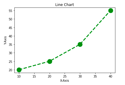
Let’s see how to customize the above-created line chart. We will be using the following properties – color: Changing the color of the linelinewidth: Customizing the width of the linemarker: For changing the style of actual plotted pointmarkersize: For changing the size of the markerslinestyle: For defining the style of the plotted lineDifferent Linestyle available Character Definition – Solid line — Dashed line -. dash-dot line : Dotted line . Point marker o Circle marker , Pixel marker v triangle_down marker ^ triangle_up marker triangle_right marker 1 tri_down marker 2 tri_up marker 3 tri_left marker 4 tri_right marker s square marker p pentagon marker * star marker h hexagon1 marker H hexagon2 marker + Plus marker x X marker D Diamond marker d thin_diamond marker | vline marker _ hline marker Example: Python3import matplotlib.pyplot as plt # initializing the datax = [10, 20, 30, 40]y = [20, 25, 35, 55] # plotting the dataplt.plot(x, y, color='green', linewidth=3, marker='o', markersize=15, linestyle='--') # Adding title to the plotplt.title("Line Chart") # Adding label on the y-axisplt.ylabel('Y-Axis') # Adding label on the x-axisplt.xlabel('X-Axis') plt.show()Output:
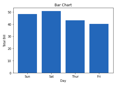
Note: For more information, refer Line plot styles in Matplotlib Bar ChartA bar chart is a graph that represents the category of data with rectangular bars with lengths and heights that is proportional to the values which they represent. The bar plots can be plotted horizontally or vertically. A bar chart describes the comparisons between the discrete categories. It can be created using the bar() method. In the below example, we will use the tips dataset. Tips database is the record of the tip given by the customers in a restaurant for two and a half months in the early 1990s. It contains 6 columns as total_bill, tip, sex, smoker, day, time, size. Example: Python3import matplotlib.pyplot as pltimport pandas as pd # Reading the tips.csv filedata = pd.read_csv('tips.csv') # initializing the datax = data['day']y = data['total_bill'] # plotting the dataplt.bar(x, y) # Adding title to the plotplt.title("Tips Dataset") # Adding label on the y-axisplt.ylabel('Total Bill') # Adding label on the x-axisplt.xlabel('Day') plt.show()Output:
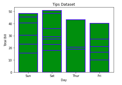
Customization that is available for the Bar Chart – color: For the bar facesedgecolor: Color of edges of the barlinewidth: Width of the bar edgeswidth: Width of the barExample: Python3import matplotlib.pyplot as pltimport pandas as pd # Reading the tips.csv filedata = pd.read_csv('tips.csv') # initializing the datax = data['day']y = data['total_bill'] # plotting the dataplt.bar(x, y, color='green', edgecolor='blue', linewidth=2) # Adding title to the plotplt.title("Tips Dataset") # Adding label on the y-axisplt.ylabel('Total Bill') # Adding label on the x-axisplt.xlabel('Day') plt.show()Output:
Note: The lines in between the bars refer to the different values in the Y-axis of the particular value of the X-axis. HistogramA histogram is basically used to represent data provided in a form of some groups. It is a type of bar plot where the X-axis represents the bin ranges while the Y-axis gives information about frequency. The hist() function is used to compute and create histogram of x. Syntax: matplotlib.pyplot.hist(x, bins=None, range=None, density=False, weights=None, cumulative=False, bottom=None, histtype=’bar’, align=’mid’, orientation=’vertical’, rwidth=None, log=False, color=None, label=None, stacked=False, \*, data=None, \*\*kwargs) Example: Python3import matplotlib.pyplot as pltimport pandas as pd # Reading the tips.csv filedata = pd.read_csv('tips.csv') # initializing the datax = data['total_bill'] # plotting the dataplt.hist(x) # Adding title to the plotplt.title("Tips Dataset") # Adding label on the y-axisplt.ylabel('Frequency') # Adding label on the x-axisplt.xlabel('Total Bill') plt.show()Output:
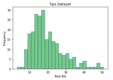
Customization that is available for the Histogram – bins: Number of equal-width bins color: For changing the face coloredgecolor: Color of the edgeslinestyle: For the edgelinesalpha: blending value, between 0 (transparent) and 1 (opaque)Example: Python3import matplotlib.pyplot as pltimport pandas as pd # Reading the tips.csv filedata = pd.read_csv('tips.csv') # initializing the datax = data['total_bill'] # plotting the dataplt.hist(x, bins=25, color='green', edgecolor='blue', linestyle='--', alpha=0.5) # Adding title to the plotplt.title("Tips Dataset") # Adding label on the y-axisplt.ylabel('Frequency') # Adding label on the x-axisplt.xlabel('Total Bill') plt.show()Output:
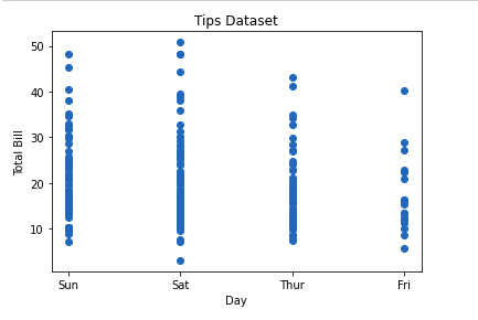
Scatter plots are used to observe relationships between variables. The scatter() method in the matplotlib library is used to draw a scatter plot. Syntax: matplotlib.pyplot.scatter(x_axis_data, y_axis_data, s=None, c=None, marker=None, cmap=None, vmin=None, vmax=None, alpha=None, linewidths=None, edgecolors=None Example: Python3import matplotlib.pyplot as pltimport pandas as pd # Reading the tips.csv filedata = pd.read_csv('tips.csv') # initializing the datax = data['day']y = data['total_bill'] # plotting the dataplt.scatter(x, y) # Adding title to the plotplt.title("Tips Dataset") # Adding label on the y-axisplt.ylabel('Total Bill') # Adding label on the x-axisplt.xlabel('Day') plt.show()Output:
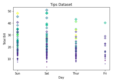
Customizations that are available for the scatter plot are – s: marker size (can be scalar or array of size equal to size of x or y)c: color of sequence of colors for markersmarker: marker stylelinewidths: width of marker borderedgecolor: marker border coloralpha: blending value, between 0 (transparent) and 1 (opaque)Python3import matplotlib.pyplot as pltimport pandas as pd # Reading the tips.csv filedata = pd.read_csv('tips.csv') # initializing the datax = data['day']y = data['total_bill'] # plotting the dataplt.scatter(x, y, c=data['size'], s=data['total_bill'], marker='D', alpha=0.5) # Adding title to the plotplt.title("Tips Dataset") # Adding label on the y-axisplt.ylabel('Total Bill') # Adding label on the x-axisplt.xlabel('Day') plt.show()Output:
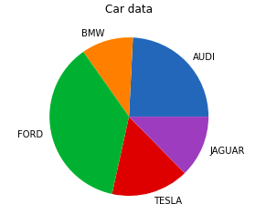
Pie chart is a circular chart used to display only one series of data. The area of slices of the pie represents the percentage of the parts of the data. The slices of pie are called wedges. It can be created using the pie() method. Syntax: matplotlib.pyplot.pie(data, explode=None, labels=None, colors=None, autopct=None, shadow=False) Example: Python3import matplotlib.pyplot as pltimport pandas as pd # Reading the tips.csv filedata = pd.read_csv('tips.csv') # initializing the datacars = ['AUDI', 'BMW', 'FORD', 'TESLA', 'JAGUAR',]data = [23, 10, 35, 15, 12] # plotting the dataplt.pie(data, labels=cars) # Adding title to the plotplt.title("Car data") plt.show()Output:
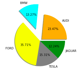
Customizations that are available for the Pie chart are – explode: Moving the wedges of the plotautopct: Label the wedge with their numerical value.color: Attribute is used to provide color to the wedges.shadow: Used to create shadow of wedge.Example: Python3import matplotlib.pyplot as pltimport pandas as pd # Reading the tips.csv filedata = pd.read_csv('tips.csv') # initializing the datacars = ['AUDI', 'BMW', 'FORD', 'TESLA', 'JAGUAR',]data = [23, 13, 35, 15, 12] explode = [0.1, 0.5, 0, 0, 0] colors = ( "orange", "cyan", "yellow", "grey", "green",) # plotting the dataplt.pie(data, labels=cars, explode=explode, autopct='%1.2f%%', colors=colors, shadow=True) plt.show()Output:
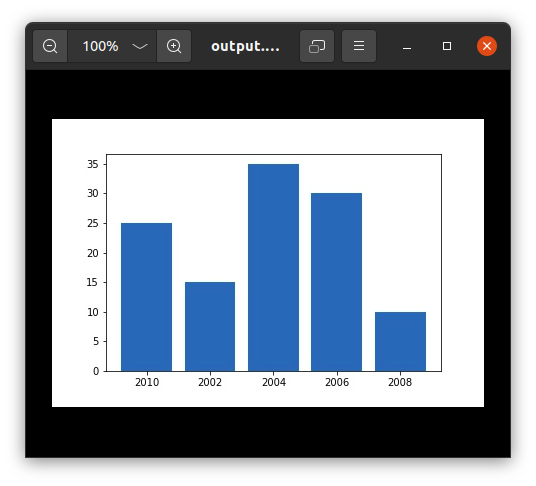
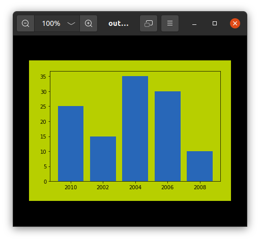
For saving a plot in a file on storage disk, savefig() method is used. A file can be saved in many formats like .png, .jpg, .pdf, etc. Syntax: pyplot.savefig(fname, dpi=None, facecolor=’w’, edgecolor=’w’, orientation=’portrait’, papertype=None, format=None, transparent=False, bbox_inches=None, pad_inches=0.1, frameon=None, metadata=None) Example: Python3import matplotlib.pyplot as plt # Creating datayear = ['2010', '2002', '2004', '2006', '2008']production = [25, 15, 35, 30, 10] # Plotting barchartplt.bar(year, production) # Saving the figure.plt.savefig("output.jpg") # Saving figure by changing parameter valuesplt.savefig("output1", facecolor='y', bbox_inches="tight", pad_inches=0.3, transparent=True)Output:
|

【本文地址】